Tag Archives: Difficulty 9
Protected: Geometric Connected Dominating Set
Pokemon
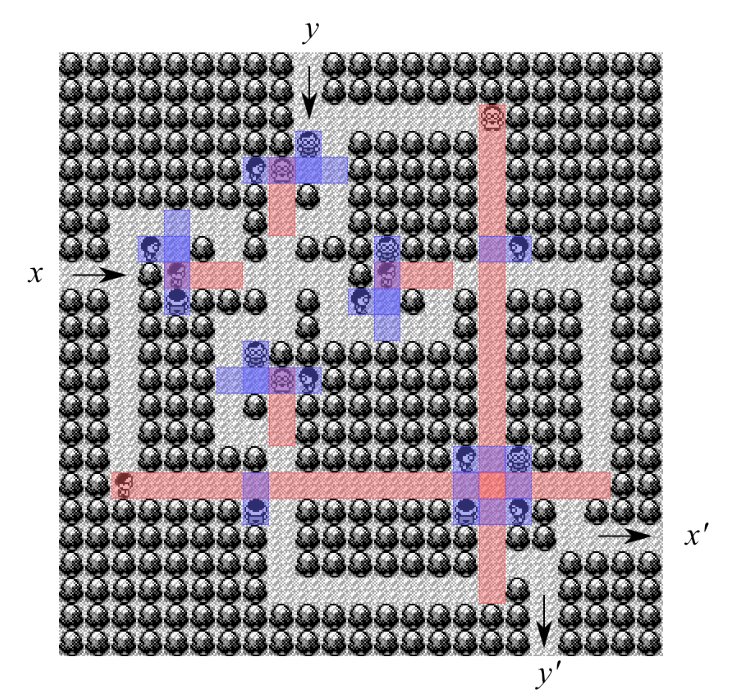
The other major reduction my student, Dan Thornton, was working on was a reduction for the old NES Pokemon game.
This is Dan’s last reduction for his independent study class. He’s going to be applying to grad schools this year- if you’re running a grad program, you should accept him!
(Over to Dan)
The Problem:
Here we prove that a generalized version of the classic Pokemon Red/Blue video game is NP-complete. Generalized Pokemon(hereafter referred to as ![]() ) asks the following question: Given a party of Pokemon and a map of trainers, can you get from the start position to the end position without having all of your Pokemon defeated in battle and continue your journey of catching them all?
) asks the following question: Given a party of Pokemon and a map of trainers, can you get from the start position to the end position without having all of your Pokemon defeated in battle and continue your journey of catching them all?
This is based off of a paper by Aloupis, Demaine, Guo, and Viglietta on classical Nintendo games.
Background:
The goal of any Pokemon game is progress through the world collecting all Pokemon to become the very best Pokemon trainer there ever was. For more background see this link. We will focus on a subproblem where there is a path filled with enemy trainers from a start point to some end point. Solving ![]() and determining if we can get to the finish from the start turns out to be NP-complete.
and determining if we can get to the finish from the start turns out to be NP-complete.
In our construction of ![]() , there are two types of enemy trainers we will encounter, Hard trainers which we will always lose against, and Easy trainers which we will always win against. The details of this construction will be described below.
, there are two types of enemy trainers we will encounter, Hard trainers which we will always lose against, and Easy trainers which we will always win against. The details of this construction will be described below.
The description:
Here we reduce ![]() from 3 SAT by building certain constructs or gadgets in
from 3 SAT by building certain constructs or gadgets in ![]() that can be used to model clauses, variables, variable assignment, and satisfiability. Then inductively using these component pieces we may build an instance of
that can be used to model clauses, variables, variable assignment, and satisfiability. Then inductively using these component pieces we may build an instance of ![]() that is logically equivalent to one from
that is logically equivalent to one from ![]() . Below is the framework that we will map components of
. Below is the framework that we will map components of ![]() on to.
on to.
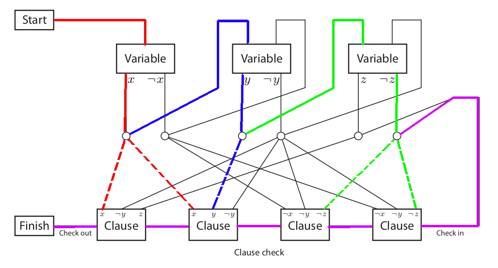
In the above figure all solid lines are single use paths, all dashed lines have no traversal limit.
The idea is that our trainer starts at the Start location and proceeds to a variable gadget, they then have an exclusive choice between two paths. One path reflects the assignment of true, the other of false. This choice will take us to a series of paths that will let us proceed to each clause the variable assignment satisfies and unlock it. Then we move on to the next variable. Eventually after proceeding through all of the variable clauses, we arrive at the Check in phase. Here we try to pass through all of the clauses, only the clauses we previously satisfied with the correct variable assignment may be passed through. Now if all clauses are satisfied, then we are able to pass through every one and arrive at the Finish state.
As an example in the above figure the colored edges give use a path that will satisfy all the clauses and pass to the Finish. The red edges show us assigning the value of true to ![]() then proceeding to the first and second clause which are satisfied by this assignment of
then proceeding to the first and second clause which are satisfied by this assignment of ![]() . The blue edges show an assignment for
. The blue edges show an assignment for ![]() and the green one for
and the green one for ![]() . It is important to note that we are unable to move backwards except on dashed edges, this prevents us from going back and attempting to correct our variable assignment.
. It is important to note that we are unable to move backwards except on dashed edges, this prevents us from going back and attempting to correct our variable assignment.
Introduction
To show equivalence we break any ![]() instance up into to following:
instance up into to following: ![]() . Here each clause is of the form:
. Here each clause is of the form:
![]() where
where
![]()
and each ![]() is a literal of the form
is a literal of the form ![]() .
.
Components
The construction of the GP instance is built out of several component pieces, each described below.
Trainer Construction
Our trainer has a single Pokemon, a Ghastly that knows only a single move– Self-Destruct, a move that when used causes the user to faint but deals massive damage to a single enemy Pokemon. If it is ever our trainer’s turn during a battle we are forced to use a move.
By the above, if we ever use a move, we lose due to us only having a single suicidal move and a single Pokemon. When we lose we are unable to move and will be unable to get to the Finish.
Hard trainers have two Snorelaxs, both of which are slower than our Ghastly, so when we go into battle against them we are forced to use self-destruct and lose. Even if we cause a single of the opponent’s Snorelax to faint we still lose the battle as they have another.
Easy trainers all have a single Electrode that only knows self-destruct and has more speed than our Ghastly, so they will always go first and destroy themselves. Now normally self destruct would also deal massive damage to our Ghastly but, because Ghastly is a ghost type Pokemon, and self-destruct is a normal type move, it will not effect our Ghastly. Thus the opposing trainer will run out of Pokemon before us, and we win.
So, we have a situation where we may encounter any number of weak trainers and win, but a battle with a strong trainer guarantees a loss.
Field of Vision
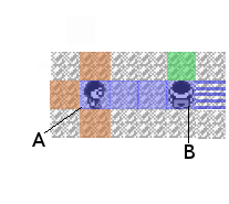
Enemy trainers have a “field of vision” of some fixed length. In the above Figure, Player A’s field of vision is given by all blue squares. Once a player enters a trainer’s field of view they will be unable to move, the enemy trainer who can see them will approach and the trainer will be forced to battle. Other enemy trainers can block a trainer’s field of view, for example the striped blue box above is no longer in trainer A’s field of view due to trainer B.
Alternatively, we may choose to force an enemy trainer to battle our trainer if we stand in any of the orange squares.
Finally, once an enemy trainer has been defeated they will remain on the square they were defeated on indefinitely, so if we challenged and beat trainer A with our trainer standing on any of the orange squares, then trainer A would stay on the exact square he is on even if our trainer moved into his field of vision (any of the solid blue squares).
To distinguish the two types of trainers hard trainers will have a blue field of vision, whereas easy trainers will have a red one.
Variable Construction
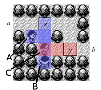
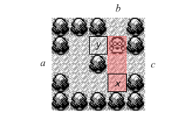
Variable assignment may be modeled using the construction in Figure 3. Here the player enters through a. The player may either choose to move to battle the enemy trainer while standing on square x or y. If our trainer battles the enemy trainer on square x then the enemy trainer will block off the c exit, and once defeated will stay there indefinitely. Alternatively if our trainer battles on square y then the defeated enemy trainer will remain where he is indefinitely and we must exit through c. So this construction therefore presents the player with an exclusive choice between two possible paths b or c.
Single Use path
In order to prevent a player from re-tracing his or her steps to access previous paths we may use the construction below. Here if we assume a player enters from a and will exit through b.
Notice that to pass from a to b our player must pass through both squares marked x and y. Notice that once we pass through y trainer C will have moved forwards to battle our trainer at y. This now means that trainer B has line of sight to x. Now because we must go through x square to get from a to b or b to a any passage through this gadget will be impossible.
Also notice that if we enter from b then we must pass through y before x and so by the same argument as above this is impossible.
Trainer A simply serves as a barrier from letting us battle trainer C from an adjacent square.
So this gadget is a single use unidirectional path.
Clauses
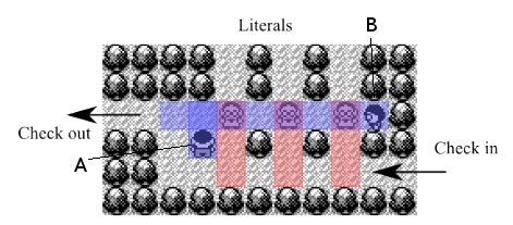
Below we illustrate a ![]() clause, each of the weak trainers is a literal.
clause, each of the weak trainers is a literal.
If the player at any time enters through any of the three literal paths from above, then they may battle a weak trainer. If a player battles any of the weak trainers then later on when the clause gadget is entered through check in then the weak trainer the player already battled will not approach the player, and will instead continue to block hard trainer B’s field of vision so that we may pass through to check out. Hard trainer A is there just to prevent re-entering the literal clauses after entering this gadget through check in.
Crossover
The crossover gadget shown below is present to deal with the issue of planarity, as there is no device in the original Pokemon games for passing “over” other portions. Then if we view the paths between gadgets as edges of a graph similar to our framework in the first figure, then without this gadget we are restricted to building planar graphs.
This gadget lets two paths cross without letting a player switch the path they are on. So if you enter from ![]() a player is forced to leave through
a player is forced to leave through ![]() and similarly for
and similarly for ![]() and
and ![]() . Each path is single use, but using the
. Each path is single use, but using the ![]() ‘s path, has no effect on our use of the
‘s path, has no effect on our use of the ![]() ‘s path and vice versa. As a result we may assume we can build a single use path between any two points.
‘s path and vice versa. As a result we may assume we can build a single use path between any two points.
Reduction
Here we reduce from an instance of ![]() . We are given a formula
. We are given a formula ![]() with the form defined in section 4. Now we build
with the form defined in section 4. Now we build ![]() into an instance of
into an instance of ![]() using the reduction framework in Figure 1 as well as our components. We also impose the restriction that in every variable gadget path
using the reduction framework in Figure 1 as well as our components. We also impose the restriction that in every variable gadget path ![]() corresponds to assigning a literal the value
corresponds to assigning a literal the value ![]() and
and ![]() corresponds to
corresponds to ![]() .
.
![]()
If we have a variable assignment ![]() that satisfies
that satisfies ![]() then by definition there is a literal
then by definition there is a literal ![]() in every clause
in every clause ![]() such that
such that ![]() satisfies
satisfies ![]() . Then in our constructed instance of
. Then in our constructed instance of ![]() we must be able to visit the literal section of every clause gadget at least once prior to arriving at the check-in phase. So it follows that we are able to battle at least 1 of the easy trainers in each clause gadget before check-in. Therefore it must be possible for us to reach the finish.
we must be able to visit the literal section of every clause gadget at least once prior to arriving at the check-in phase. So it follows that we are able to battle at least 1 of the easy trainers in each clause gadget before check-in. Therefore it must be possible for us to reach the finish.
![]()
If it is possible for our trainer to get from start to finish, then again by the framework in Figure 1 we must be able to battle an easy trainer in each of our clause gadgets. To reach these clause gadgets the trainer had to make an exclusive decision in each variable gadget. This choice corresponds to a literal assignment. So the path our trainer takes through the variable gadgets, and then through the clause gadgets to the finish gives us an assignment of literals such that every clause is satisfied. Obviously this corresponds to an assignment that satisfies ![]() .
.
(Back to me)
Difficulty: 9. This isn’t that hard to understand, but there are lots of details that are needed- having to position the trainers in exactly the right position for it all to work.
Minimum Inferred Finite State Automaton
Here’s the actual problem my student Dan Thornton spent most of his semester trying to understand and prove. It’s pretty crazy.
The problem: Automaton Identification from Given Data. We abbreviate it “AutID”. G&J call this problem “Minimum Inferred Finite State Automaton” and it is problem AL8 in the appendix.
The description: Given a finite set of data, is it possible to build a deterministic finite automata of ![]() or fewer states that agrees with the data?
or fewer states that agrees with the data?
Prior to giving a description of this problem we must introduce a few concepts and definitions. We want to construct a finite automation, this means a Mealy model deterministic finite automata. Formally a 6-tuple of the form
![]()
 is the input alphabet, where
  is an individual character, and
  is a string.
 the set of states in the model.
  refers to an individual state.
  may equivalently be referred to as the set
 ![Rendered by QuickLaTeX.com S_{[s]}](https://npcomplete.owu.edu/wp-content/ql-cache/quicklatex.com-b8150e1cdd7a6d8b6757709c274c72aa_l3.png) of all equivalence classes
of all equivalence classes ![Rendered by QuickLaTeX.com [s]_{\overline{u}}](https://npcomplete.owu.edu/wp-content/ql-cache/quicklatex.com-92de2112a12b2d8a768786943b94f7f2_l3.png) , with representative element
, with representative element  . Each equivalence class is a set of all input strings
  such that
  .
. the output alphabet, where
  is a individual character,
  .
. is the transition function.
 is the output function.
- Both of the above functions may be extended in a natural way so that
 and
and  respectively. Usage should be clear from context.
- Both of the above functions may be extended in a natural way so that
 is the start state.
We use the standard convention that ![]() refers to the empty string of no characters.
refers to the empty string of no characters.
A black box is similar to an ‘unknown’ Mealy model with the restriction that for any input string ![]() we only get to see the last output character
we only get to see the last output character ![]() returns. Consider the following black box. With input alphabet
returns. Consider the following black box. With input alphabet ![]() and output alphabet
and output alphabet ![]() .
.
So if the above known black box was passed the string ![]() the complete Mealy model’s output function would give us back the string
the complete Mealy model’s output function would give us back the string ![]() where as the black box would only give us back
where as the black box would only give us back ![]() .
.
Now our above finite automata is constructed using data we are given, here we assume that data is a set ![]() of finite pairs of the form
of finite pairs of the form ![]() .
.
![]() such that
such that ![]() is not empty and
is not empty and ![]() for
for ![]() .
.
An automata ![]() agrees with data
agrees with data ![]() if for every datum
if for every datum ![]() , the final output character of
, the final output character of ![]() .
.
Formal Problem Statement:
Given input alphabet ![]() , output alphabet
, output alphabet ![]() and data, a set
and data, a set ![]() of finite pairs determine if an automation of
of finite pairs determine if an automation of ![]() or fewer states exists that agrees with D.
or fewer states exists that agrees with D.
The Reduction:
The reduction by Gold uses Monotone EQ SAT. So we are given a conjunction of clauses ![]() where each clause in
where each clause in ![]() contains all negated or non-negated variables
contains all negated or non-negated variables ![]() and the number of clauses and variables is equal, is there an assignment of the variables so that
and the number of clauses and variables is equal, is there an assignment of the variables so that ![]() is satisfied? Our instance will have
is satisfied? Our instance will have ![]() clauses and variables. Clauses will be numbered
clauses and variables. Clauses will be numbered ![]() and variables will be numbered
and variables will be numbered ![]() .
.
In the above instance of Monotone EQ SAT we do not have a variable ![]() . Indices in our reduction will sometimes force us to reference
. Indices in our reduction will sometimes force us to reference ![]() . We may think of this variable as simply a place holder for
. We may think of this variable as simply a place holder for ![]() .
.
The idea behind this reduction is that we may encode our instance of Monotone EQ SAT into data ![]() in such a way that if we can create a finite automata from our encoding, then we can use it to obtain a solution to the instance of Monotone EQ SAT if one exists.
in such a way that if we can create a finite automata from our encoding, then we can use it to obtain a solution to the instance of Monotone EQ SAT if one exists.
Aut ID construction:
Here we transform our instance of Monotone EQ SAT into data ![]() , to do so we need the following functions:
, to do so we need the following functions:
![]()
![]()
The bounds on the above functions are a result of our numbering of clauses ![]() and
and ![]() . Note that
. Note that ![]() is really a placeholder for
is really a placeholder for ![]() .
.
Given a propositional formula ![]() which is an instance of MonotoneEQ SAT we encode it by the following:
which is an instance of MonotoneEQ SAT we encode it by the following:
- The variables of
 are encoded by the set
 . Here each
  corresponds to the element
  where
where  is an element of the output alphabet,
  .
. - We encode the clauses
 of
of  by
by  for
for  ,
,  . Here each clause has a \textit{identifying tag},
  , then the
  term is used specify a particular variable,
  . Importantly, datum in this set for which
  returns
  are thrown out.
- Each clause encoding
 will be
  only if clause
  does not contain variable
  , otherwise
  will be
  and is thrown out.
- Each clause encoding
- We then encode whether each clause is a set of all negated, or non-negated variables.
 for
for  .
.
As a simple example we convert to data the following formula
![]()
So after our conversion we get:
Aut ID instance
Now we create an instance of ![]() by letting
by letting ![]() be the number of variables
be the number of variables ![]() and
and ![]() .
.
True{Aut ID} ![]() True{Monotone EQ SAT}
True{Monotone EQ SAT}
Now we may assume that we have a finite automata ![]() that agrees with the data in
that agrees with the data in ![]() . Now we may use the transition function
. Now we may use the transition function ![]() and the output function
and the output function ![]() to deduce properties of
to deduce properties of ![]() .
.
Let ![]() be
be ![]() , this is the state that
, this is the state that ![]() is in after receiving the input string
is in after receiving the input string ![]() .
.
A splitting string of ![]() and
and ![]() is a string
is a string ![]() so that
so that ![]() differs from
differs from ![]() . If such a string exists then obviously
. If such a string exists then obviously ![]() . If two states do not have splitting string then they are equivalent
. If two states do not have splitting string then they are equivalent
We define variable states as follows, a variable ![]() has the encoding
has the encoding ![]() , so
, so ![]() is
is ![]() ‘s variable state, we will sometimes refer to this as
‘s variable state, we will sometimes refer to this as ![]() .
.
Clause states are defined in a manner similar to variable states. A clause ![]() corresponds to the identifying tag in the encoding of
corresponds to the identifying tag in the encoding of ![]() or
or ![]() , so
, so ![]() is
is ![]() ‘s clause state, we will sometimes refer to this as
‘s clause state, we will sometimes refer to this as ![]() .
.
In the following theorems we shall talk of assignment of clause state ![]() to variable state
to variable state ![]() , this means that these two states are equivalent or alternatively that there does not exist a splitting string of
, this means that these two states are equivalent or alternatively that there does not exist a splitting string of ![]() and
and ![]() .
.
Theorem 1:All variable states are different.
Proof. We assume two variable states are equal ![]() and
and ![]() where
where ![]() . Then in the encoding of
. Then in the encoding of ![]() we get
we get ![]() and
and ![]() respectively. But now we may define the splitting string
respectively. But now we may define the splitting string ![]() . The final element of
. The final element of ![]() is defined in our data
is defined in our data ![]() as
as ![]() . By a similar argument we get
. By a similar argument we get ![]() where
where ![]() , in our data this corresponds to one of the entries
, in our data this corresponds to one of the entries ![]() . Our automata
. Our automata ![]() must agree with the data, so as a result these states
must agree with the data, so as a result these states ![]() and
and ![]() cannot be equal. Thus we have reached a contradiction.
cannot be equal. Thus we have reached a contradiction. ![]()
Theorem 2: Each state in our finite automata ![]() corresponds to exactly one variable.
corresponds to exactly one variable.
Proof. The above follows by the pigeonhole principle, as ![]() has exactly
has exactly ![]() states, there are
states, there are ![]() variable states, and by Theorem 1, no two variable states are equal.
variable states, and by Theorem 1, no two variable states are equal. ![]()
By the above we may talk about the states of ![]() in term of the variable each state corresponds to.
in term of the variable each state corresponds to.
Theorem 3: If clause state ![]() and variable state
and variable state ![]() are equal, Then clause
are equal, Then clause ![]() contains variable
contains variable ![]() .
.
Proof. Assume ![]() =
= ![]() and
and ![]() is not contained in
is not contained in ![]() . Once again we have the following encodings
. Once again we have the following encodings ![]() and
and ![]() that were defined in our construction of
that were defined in our construction of ![]() . Now we may define a splitting string
. Now we may define a splitting string ![]() . When we append the splitting string to each of the above encodings we get
. When we append the splitting string to each of the above encodings we get ![]() and
and ![]() . Both of these strings are defined in our data
. Both of these strings are defined in our data ![]() as
as ![]() and
and ![]() respectively, and by our assumption that
respectively, and by our assumption that ![]() is not contained in
is not contained in ![]() ,
, ![]() So by the a conclusion identical to that of Theorem 1,
So by the a conclusion identical to that of Theorem 1, ![]() and our theorem follows.
and our theorem follows. ![]()
Theorem 4:No two clause states ![]() and
and ![]() may be equal if they are of opposite composition, meaning one has all negated variables, and the other all un-negated variables.
may be equal if they are of opposite composition, meaning one has all negated variables, and the other all un-negated variables.
Proof. Once again we proceed by contradiction, assume ![]() and that
and that ![]() ,
, ![]() are of opposite composition. Once again we get each clauses encoding
are of opposite composition. Once again we get each clauses encoding ![]() and
and ![]() respectively. Now we may define the splitting string
respectively. Now we may define the splitting string ![]() . Looking at the final character output by
. Looking at the final character output by ![]() we see
we see ![]() and
and ![]() . It follows that
. It follows that ![]() as
as ![]() and
and ![]() are of opposite composition. Thus we arrive at a contradiction.
are of opposite composition. Thus we arrive at a contradiction.![]()
Theorem 5: ![]() gives us a solution to
gives us a solution to ![]() our instance of
our instance of ![]() .
.
Proof. By Theorem 2 every clause state must be assigned to a single variable state, notice this does not mean only a single assignment is possible but just the given automata ![]() will give a single assignment. By Theorem 1 no clause may be assigned more than one variable state. By Theorem 3 a clause may be assigned to a variable state only if the clause contains the variable. So we see that our automata
will give a single assignment. By Theorem 1 no clause may be assigned more than one variable state. By Theorem 3 a clause may be assigned to a variable state only if the clause contains the variable. So we see that our automata ![]() assigns clauses to the variables that could potentially satisfy them. Furthermore by Theorem 4, each variable state is given clauses of only one composition, so there is an obvious variable assignment to satisfy all of the clause states equal to a given variable state.
assigns clauses to the variables that could potentially satisfy them. Furthermore by Theorem 4, each variable state is given clauses of only one composition, so there is an obvious variable assignment to satisfy all of the clause states equal to a given variable state. ![]()
True{Monotone EQ SAT} ![]() True{Aut ID}
True{Aut ID}
Now we assume there exists a mapping ![]() that satisfies our instance of Monotone EQ SAT,
that satisfies our instance of Monotone EQ SAT, ![]() with
with ![]() clauses and variables. From this mapping we build a finite automata
clauses and variables. From this mapping we build a finite automata ![]() that agrees with all data
that agrees with all data ![]() .
.
We let ![]() ‘s 0-transitions refer to transitions on input 0. Similarly 1-transitions refer to the transitions on input 1.
‘s 0-transitions refer to transitions on input 0. Similarly 1-transitions refer to the transitions on input 1.
So first we define all 1-transitions as given in the following example automata, obviously such transitions will satisfy all data in ![]() .
.
Now for ![]() to satisfy all of the data in
to satisfy all of the data in ![]() we notice by Theorems 3 and 4 above mapping each clause to the variable state that satisfies it seems like a natural thing to do. We may determine this mapping of clauses to the variables that satisfy them from our truth assignment that satisfies
we notice by Theorems 3 and 4 above mapping each clause to the variable state that satisfies it seems like a natural thing to do. We may determine this mapping of clauses to the variables that satisfy them from our truth assignment that satisfies ![]() ,
, ![]() .
.
Such mappings may be added to ![]() by noticing the following, as soon as we encounter a 0 in input we must transition to a clause state. So we may define a 0-transition for every state in
by noticing the following, as soon as we encounter a 0 in input we must transition to a clause state. So we may define a 0-transition for every state in ![]() that maps the clause state
that maps the clause state ![]() (which recall corresponds to the string
(which recall corresponds to the string ![]() ) to the variable state
) to the variable state ![]() that satisfies it. When adding 0-transitions we must be careful as if clause
that satisfies it. When adding 0-transitions we must be careful as if clause ![]() is satisfied by variable
is satisfied by variable ![]() then in order to agree with the data in
then in order to agree with the data in ![]() we really should map
we really should map ![]() to variable
to variable ![]() due to the definition of
due to the definition of ![]() .
.
Now we must assign an output to each of these 0-transitions. To do so we iterate through every clause state ![]() by sequentially considering
by sequentially considering ![]() . At each clause state we assign the output of the 0-transition starting at this state to be
. At each clause state we assign the output of the 0-transition starting at this state to be ![]() . Notice that if two clause states
. Notice that if two clause states ![]() and
and ![]() are identical, then they must both be satisfied by the same variable and so therefore
are identical, then they must both be satisfied by the same variable and so therefore ![]() .
.
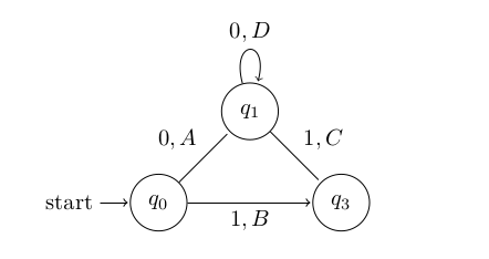
Below is an example of adding such a 0-transition and assigning its output:
The Blue edge is the zero transition added that maps the clause state ![]() ,which corresponds to the string
,which corresponds to the string ![]() , to the variable state
, to the variable state ![]() . Semantically this means that the variable
. Semantically this means that the variable ![]() satisfies this clause.
satisfies this clause.
The Red edge shows us adding the output value of a 0-transition, as from the above blue edge we know ![]() corresponds to the clause
corresponds to the clause ![]() ‘s clause state, so to the zero transition from this clause state will have output
‘s clause state, so to the zero transition from this clause state will have output ![]() .
.
Theorem 6: Our constructed automata ![]() agrees with all
agrees with all ![]()
Proof. This is quite obvious from our example of ![]() in Figure 1. We have defined all the
in Figure 1. We have defined all the ![]() transitions, and notice that the final output of all
transitions, and notice that the final output of all ![]() if
if ![]() and
and ![]() this exactly matches our data
this exactly matches our data ![]() .
. ![]()
Theorem 7: Our constructed automata ![]() agrees with all
agrees with all ![]()
Proof:Here we consider the final character output of ![]() for all encodings of fixed clause
for all encodings of fixed clause ![]() , these encodings are precisely the
, these encodings are precisely the ![]() for
for ![]() . Now with the addition of the
. Now with the addition of the ![]() -transitions, we transition into
-transitions, we transition into ![]() , and from this state we only worry about
, and from this state we only worry about ![]() -transitions. Recall that in our definition of
-transitions. Recall that in our definition of ![]() , all datum are of the form
, all datum are of the form ![]() . In
. In ![]() there is a single
there is a single ![]() -transition that outputs the non-zero value
-transition that outputs the non-zero value ![]() . To agree with
. To agree with ![]() it is sufficient to make sure that this non-zero output occurs for an input string not in
it is sufficient to make sure that this non-zero output occurs for an input string not in ![]() .
.
From our assignment of ![]() -transitions defined above this singular
-transitions defined above this singular ![]() -transition that outputs
-transition that outputs ![]() will occur for the variable
will occur for the variable ![]() that satisfies
that satisfies ![]() , so then
, so then ![]() must be in
must be in ![]() . So
. So ![]() will give the datum (
will give the datum (![]() ,1). Now notice the corresponding entry in
,1). Now notice the corresponding entry in ![]() as defined by
as defined by ![]() would be (
would be (![]() ,
,![]() ), but all of these datum were removed from
), but all of these datum were removed from ![]() . So the sufficiency condition above is satisfied.
. So the sufficiency condition above is satisfied. ![]()
Theorem 8 :Our constructed automata ![]() agrees with all
agrees with all ![]()
Proof: The manner in which we defined our 0 transitions explicitly involved a ![]() term, so for any clause state
term, so for any clause state ![]() , now a 0 transition as defined above will output
, now a 0 transition as defined above will output ![]() which will obviously agree with
which will obviously agree with ![]()
By Theorem 6, Theorem 7, and Theorem 8. We conclude that ![]() will agree with data
will agree with data ![]()
(Back to me)
Difficulty: 9. This is basically the reduction in the Gold paper, though Dan reorganized it a bunch to make it fit our format, and be more understandable. But the formatting of the various variables, the fact that you need to define the IF function on variable k to talk about zl-k instead of zk, and the three different kinds of test data all make this super hard to understand. In some ways, I wonder if this should be a 10, given the work we did on it. But I’m saving the 10’s for things that are truly impenetrable, and we did manage to figure this one out.
